Hi there, and welcome. This content is still relevant,
but fairly old. If you are interested in keeping up-to-date with similar
articles on profiling, performance testing, and writing performant
code, consider signing up to the Four Steps to Faster Software newsletter. Thanks!
In my last post, I focussed on how to go about analysing your application's inbound traffic in order to create a simulation for performance testing. One part of the analysis was determining how long to leave between each simulated message, and we saw that the majority of messages received by LMAX have less than one millisecond between them.
Using this piece of data to create a simulation doesn't really make sense - if our simulator should send messages with zero milliseconds delay between each, it will just sit in a loop sending messages as fast as possible. While this will certainly stress your system, it won't be an accurate representation of what is happening in production.
The appearance of zero just points to the fact that we are not looking close enough at the source data. If milliseconds are not precise enough to measure intervals between messages, then we need to start using microseconds. If you are using something like pcap or an application such as tcpdump to capture production traffic, then this is easy since each captured packet will be stamped with a microsecond precision timestamp by default (see pcap-tstamp for timestamp sources).
Firstly, a reminder of how the distribution appeared at the millisecond level. Note the log-scale on the Y-axis, indicating that most sequential messages had 0 - 10 milliseconds between them:

At microsecond precision, using 10 microsecond buckets, almost all datapoints are under 100 microseconds:

This is slightly easier to see when the log scale is removed from the Y axis:

It is clear from these charts that we have a broad range of message intervals under one millisecond, with most occurrences under 100 microseconds. Looking at the raw data confirms this:
Using histograms is a useful way to visually confirm that your analysis is using the right level of detail. As long as the peak of the histogram is not at zero, then you can be more confident that you have useful data for building a simulation.
Using this more detailed view, we know that our model will need to generate sequential messages with an interval of 0 to 80 microseconds most of the time with a bias towards an interval of 50 microseconds.
Removing the log-scale on the axes, and zooming in on the interesting intervals, it is easier to see that messages also arrive in bursts every 100 - 250 milliseconds:

Are these pauses between messages uniformly spread out over time, or do they follow a repeating pattern? To answer this question, we can build a histogram plotting arrival millisecond within a second - this should help to identify messages that are arriving at the larger intervals.
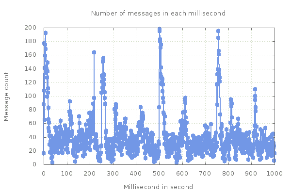
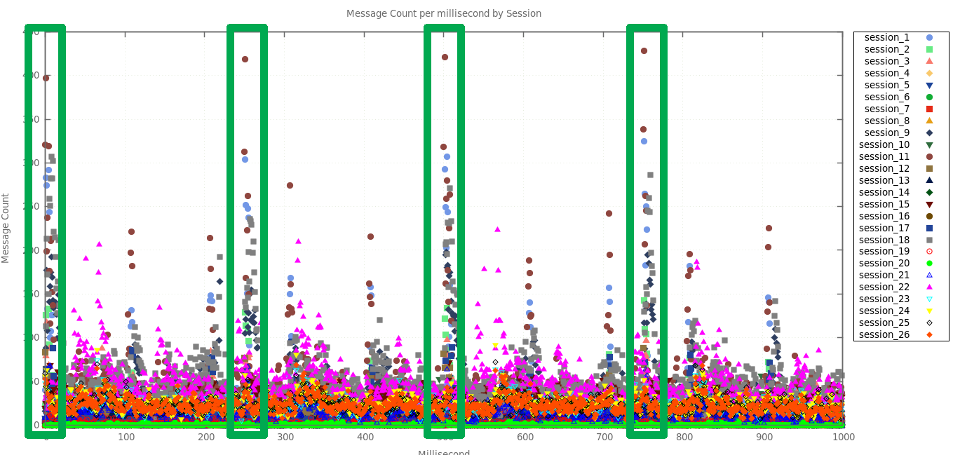
There are obvious bursts of messages at 0, 250, 500, 750 milliseconds into each second, and to a lesser extent every 100 milliseconds. This tells us that our inbound traffic is quite bursty, and that our simulation will need to replicate this behaviour to be realistic. The previous chart is only for a single session, but if we generate the same chart for all sessions, this behaviour is even more pronounced:


We found that this pattern of behaviour was probably down to our market-makers' own data sources. Each of them likely receives a market-data feed from one of several primary trading venues, who publish price updates every 250 milliseconds/100 milliseconds or so. The bursts we see in inbound traffic are down to our market-makers' algorithms reacting to their inputs.
Going to this level of detail allowed us to make sure that our performance tests were truly realistic, and identified a previously unknown aspect of user behaviour. This in turn gives us confidence that we can continue to plan for future capacity by running production-like loads in our performance test environment at ten times the current production throughput rate.
As stated in a previous post, this is an iterative process as part of our continuous delivery pipeline, so we will continue to analyse and monitor user behaviour. There are no doubt many more details that we have not yet discovered.
Follow @epickrram
Using this piece of data to create a simulation doesn't really make sense - if our simulator should send messages with zero milliseconds delay between each, it will just sit in a loop sending messages as fast as possible. While this will certainly stress your system, it won't be an accurate representation of what is happening in production.
The appearance of zero just points to the fact that we are not looking close enough at the source data. If milliseconds are not precise enough to measure intervals between messages, then we need to start using microseconds. If you are using something like pcap or an application such as tcpdump to capture production traffic, then this is easy since each captured packet will be stamped with a microsecond precision timestamp by default (see pcap-tstamp for timestamp sources).
Finding the right level of detail
Looking at inbound message intervals for a single session, but this time considering microsecond precision, a different picture emerges.Firstly, a reminder of how the distribution appeared at the millisecond level. Note the log-scale on the Y-axis, indicating that most sequential messages had 0 - 10 milliseconds between them:

At microsecond precision, using 10 microsecond buckets, almost all datapoints are under 100 microseconds:

This is slightly easier to see when the log scale is removed from the Y axis:

It is clear from these charts that we have a broad range of message intervals under one millisecond, with most occurrences under 100 microseconds. Looking at the raw data confirms this:
interval (us)    count
            0     1591
           10      611
           20     1017
           30     1243
           40     3890
           50     6167
           60     3349
           70     1655
           80      907
           90      519
          100      374
          110      291
          120      254
          130      193
          140      184
          150      156
          160      145
          170      138
          180      114
          190      111
Using histograms is a useful way to visually confirm that your analysis is using the right level of detail. As long as the peak of the histogram is not at zero, then you can be more confident that you have useful data for building a simulation.
Using this more detailed view, we know that our model will need to generate sequential messages with an interval of 0 to 80 microseconds most of the time with a bias towards an interval of 50 microseconds.
Microbursts
Examining the histogram of millisecond message intervals above, it's clear that the distribution doesn't follow a smooth curve. The chart suggests that alongside messages that arrive very close together, we also receive a number of messages with an interval on the order of hundreds of milliseconds.Removing the log-scale on the axes, and zooming in on the interesting intervals, it is easier to see that messages also arrive in bursts every 100 - 250 milliseconds:

Are these pauses between messages uniformly spread out over time, or do they follow a repeating pattern? To answer this question, we can build a histogram plotting arrival millisecond within a second - this should help to identify messages that are arriving at the larger intervals.

There are obvious bursts of messages at 0, 250, 500, 750 milliseconds into each second, and to a lesser extent every 100 milliseconds. This tells us that our inbound traffic is quite bursty, and that our simulation will need to replicate this behaviour to be realistic. The previous chart is only for a single session, but if we generate the same chart for all sessions, this behaviour is even more pronounced:
Messages received at each millisecond over time, showing 250ms bursts

Messages received at each millisecond over time, showing 100ms bursts
We found that this pattern of behaviour was probably down to our market-makers' own data sources. Each of them likely receives a market-data feed from one of several primary trading venues, who publish price updates every 250 milliseconds/100 milliseconds or so. The bursts we see in inbound traffic are down to our market-makers' algorithms reacting to their inputs.
Conclusion
The devil is in the detail - it is easy to make assumptions about how users interact with your system, given a granular overview of such metrics as requests per second but, until a proper analysis is carried out, the nature of user traffic patterns cannot be more than guessed at.Going to this level of detail allowed us to make sure that our performance tests were truly realistic, and identified a previously unknown aspect of user behaviour. This in turn gives us confidence that we can continue to plan for future capacity by running production-like loads in our performance test environment at ten times the current production throughput rate.
As stated in a previous post, this is an iterative process as part of our continuous delivery pipeline, so we will continue to analyse and monitor user behaviour. There are no doubt many more details that we have not yet discovered.
Follow @epickrram